Dynamic topography and sediment routing systems

Xuesong Ding, Tristan Salles, Nicolas Flament, Claire Mallard, Patrice Rey

Software Used:

Badlands 1.0

Dynamic topography due to mantle flow contributes to shaping Earth’s evolving landscapes by affecting sediment routing, which has rarely been explored in source-to-sink contexts. Here, we design a generic model to investigate the impact of dynamic topography on both landscape evolution and stratigraphic formations. We find that (1) Dynamic topography affects all the segments of a source-to-sink system. It induces significant reorganizations of river networks and drives complex erosion and sediment routing responses in the source region; (2) The migrating dynamic topography results in variations in sediment supply, depending on the relative directions between dynamic topography propagation and sediment transport; (3) Variations in sediment supply driven by the migrating dynamic topography contribute to the formation of diachronous unconformities along continental margins.

Model Setup:

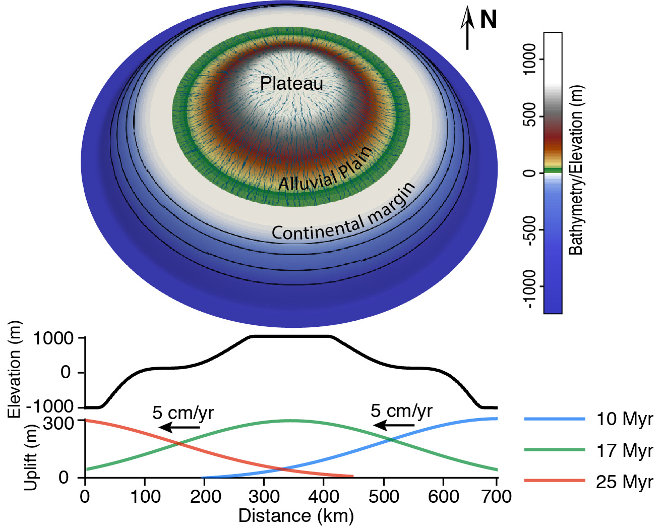Model setup of a generic case showing a wave of positive dynamic topography migrating under a fixed circular continent. The circular continent is 700 km in diameter with a spatial resolution of 1 km. Its initial landscape of the continent consists of a central plateau (source area) surrounded by an alluvial plain (transfer zone) and a continental margin (sink area). A sinusoidal wave of positive dynamic topography with a wavelength of 1000 km and amplitude of 300 m propagating to the west at 5 cm/yr is considered.

Conditions:

Variables	Parameter	value
Non Marine Erodibility	K_e	2.e-7
Rainfall	P [m/a]	1.0
(Rainfall * Area) exponent m	m	0.5
Slope exponent n	n	1.0
Slope Minimum for Flood-plain Deposition	slp_cr	0.001
Non-Marine % Max Deposition	perc_dep	0.5
Land sed. Transport by River	criver	10
Land sed. Transport by Wind	caerial	0.001
Lake/Sea sed. Transport by Currents	cmarine	0.005
No. Time Steps To Distribute Marine Deposits	diffnb	5
Marine % Max Deposition	diffprop	0.4

Results:

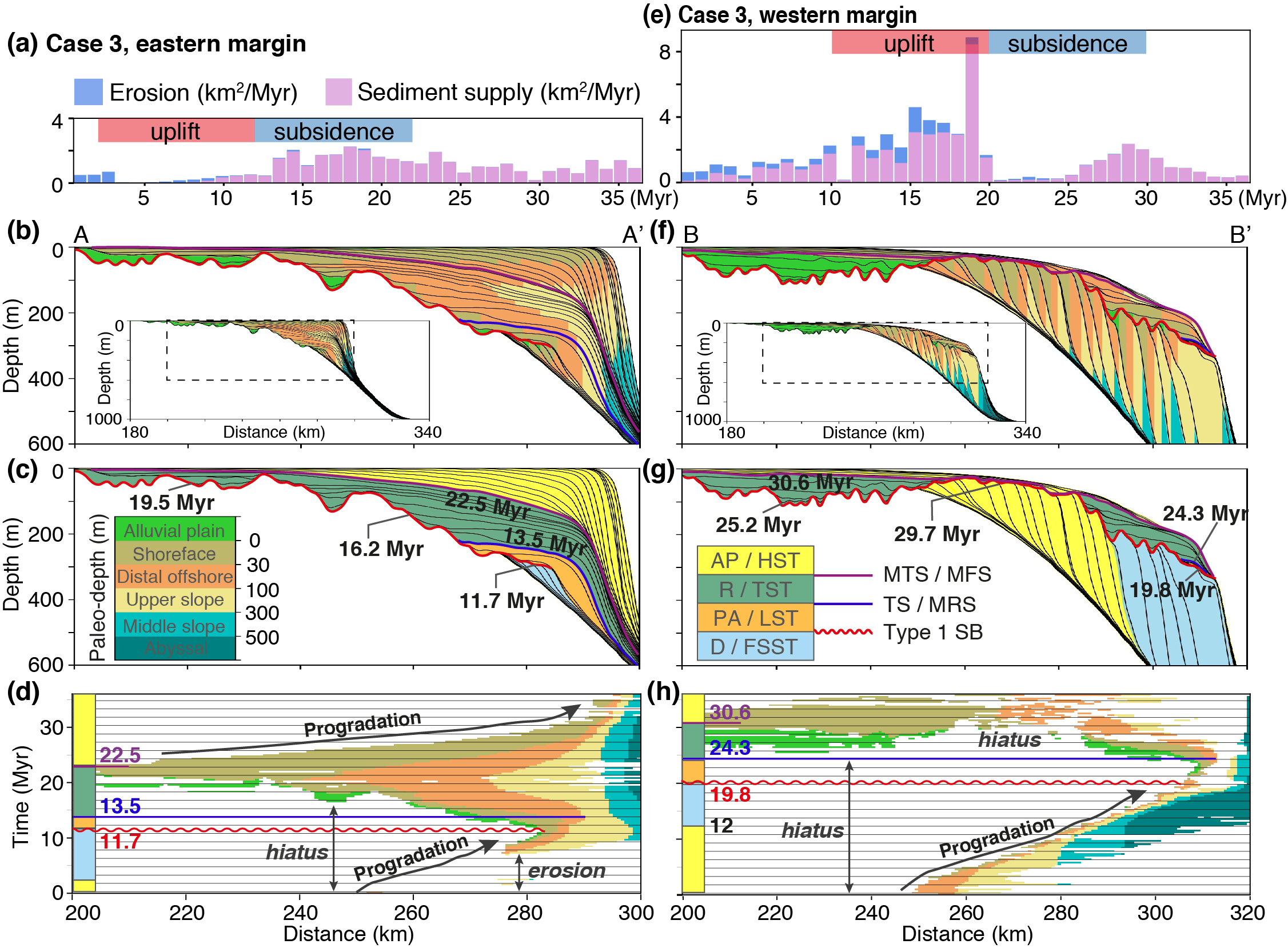(a) Sediment supply histories and erosion of stratigraphic layers, stratal stacking patterns represented by (b) depositional environments, (c) interpreted systems tracts, and (d) Wheeler diagrams reconstructed on the eastern margin. (e-h) Same for the western margin. Paleo-depth is assumed to be a proxy for depositional environments, including alluvial plain (>0 m), shoreface (or delta front, 0-30 m), distal offshore (or prodelta, 30-100 m), upper slope (100-300 m), middle slope (300-500m) and abyss (>500 m). Key stratigraphic surfaces and their timing are indicated in c, d, g and h. Systems tracts are interpreted for Case 3 with abbreviations: A - aggradation, P - progradation, R - retrogradation, D - degradation, HST - highstand systems tract, TST - transgressive systems tract, LST - lowstand systems tract, FSST - falling-stage systems tract, MTS - maximum transgressive surface, MFS - maximum flooding surface, TS – transgressive surface, MRS - maximum regressive surface, SB - sequence boundary.

Citation:

Submitted to Geophysics Research Letter